[Overall_position Age_position Age_total Name Age Gender Town State Ascent Descent Total] ...
= textread('PikesPeakMarathon2007.txt', '%d %d%*c%d %24c %d %c %15c %2c %7c %7c %7c');
Do not attempt to understand this textread() command at this time. We will study how to read data from a file later in the semester.
The column vectors that are created by the statement above are called "parallel arrays" because the data on row j of one array is related to the data on the jth row of all the other arrays. The arrays hold the following information:
| Row vector | Description | Size (Type) |
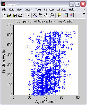
| Overall_position | The runner's finishing place (e.g., 1st, 2nd, 3rd, etc.) | 882x1 (double) |
| Age_position | The runner's finishing place in their age category | 882x1 (double) |
| Age_total | The total number of runners in this runner's age category | 882x1 (double) |
| Name | The runner's name | 882x24 (char) |
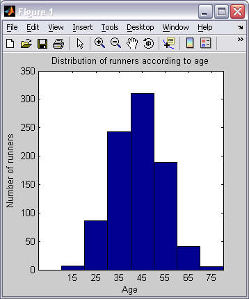
| Age | The runner's age | 882x1 (double) |
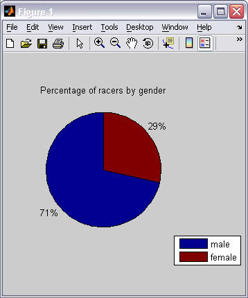
| Gender | The runner's gender | 882x1 (char) |
| Town | The runner's home town | 882x7 (char) |
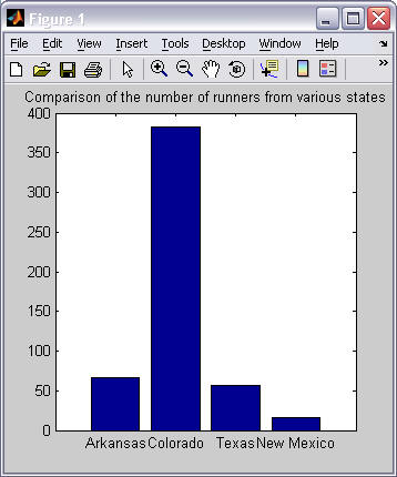
| State | The runner's home state (or country) | 882x2 (char) |
| Ascent | The time it took for the runner to get to the top of Pikes Peak | 882x7 (char) |
| Descent | The time it took for the runner to get down from the top of Pikes Peak | 882x7 (char) |
| Total | The total race time for the runner | 882x7 (char) |
% wait for user to press enter, then close the figure window
Wait = input('Press enter to continue.', 's');
close()
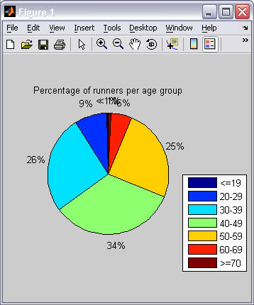
- under 20
- 20-29
- 30-39
- 40-49
- 50-59
- 60-69
- 70 and over